What's a quantum computer (draft)

Published: 26/06/2026 — Updated: 03/07/2026

In short, a quantum computer is a device that leverages the principles of quantum mechanics to execute algorithms.

Despite popular belief, a quantum computer is not inherently more capable than a classical one from a strict computability perspective¹. Any problem solvable by a quantum computer can theoretically be solved by a classical one. The true differentiator lies in the type of problems each can solve efficiently, aka computational complexity².

It is widely believed that there is a class of problems that can be solved efficiently (in polynomial time) on quantum computers, but not on classical ones. This complexity class is formally known as BQP.

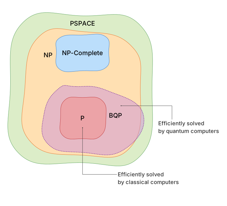
Some canonical examples of such problems are:

• Integer factoring via Shor’s algorithm.
  • Exponential speed-up.
• Unstructured search via Grover’s algorithm.
  • Quadratic speed-up³.
• Computing expectation values of a solution to a linear system of equations via the HHL algorithm.
  • Exponential speed-up⁴.

However, it is important to remark that the strict separation of these complexity classes remains a formally unproven conjecture⁵.

Beyond time complexity, quantum computers can also offer a space (memory) advantage. For instance, simulating quantum mechanical systems classically requires memory that scales exponentially, $\mathcal{O}(2^n)$, for an $n$-qubit system.

To put this into perspective, storing the state of just 50 qubits classically using 16-bit floating-point precision (float16) requires representing $2^{50}$ complex amplitudes, demanding roughly 4.5 Petabytes of RAM. A quantum computer requires exactly 50 qubits to natively hold this same state, yielding an exponential saving in memory.

Notably, this capacity is hidden behind a fundamental limitation: the readout cost. While a quantum computer can efficiently represent massive amounts of data in superposition, quantum mechanics forbids us from directly reading the full encoded information. We can access this information only by measuring, which collapses the system and yields a single probabilistic sample according to the $2^n$ probability amplitudes. If our goal is to know the full state, we have to do quantum state tomography, which has an exponential measurement cost, roughly $\mathcal{O}(4^n)$.

To understand what this precisely means, we’ll take a brief look into the mathematical formalism.

A brief look into the mathematical formalism

As you likely know, the fundamental unit of quantum computing is the qubit. Conceptually, a qubit is a mathematical object defined by two key properties: it has two distinct states, and it has the capacity to display phenomena from quantum mechanics. While qubits can be physically realized in various ways—such as superconducting circuits or trapped ions—they all share this exact foundation.

Usually, the two basis states of a qubit are represented as column vectors:

$|0\rangle=\begin{pmatrix}1 \\ 0\end{pmatrix}\quad \quad |1\rangle=\begin{pmatrix}0 \\ 1\end{pmatrix}$

These are equivalent to the 0 and 1 state of a classical bit.

A qubit can exist in a superposition, which is simply a linear combination of these basis states:

$|\psi\rangle = \alpha|0\rangle + \beta|1\rangle$

where the coefficients are complex numbers and are subject to the normalization constraint $|\alpha|^2+|\beta|^2=1$.

These coefficients, $\alpha$ and $\beta$, are the amplitudes and dictate the probability of measuring each respective state. When we measure a qubit, we will observe $|0\rangle$ (a bit equaling zero) with probability $|\alpha|^2$ and $|1\rangle$ (a bit equaling one) with probability $|\beta|^2$. The outcome of measuring a qubit is a bit; however, unlike classical probabilistic systems, the state is fundamentally indeterminate until the exact moment of measurement.

To manipulate the quantum state, we apply quantum operators. These operators are mathematically represented by unitary matrices, which allow us to perform linear transformations on the amplitudes $\alpha$ and $\beta$.

The most common framework for thinking of quantum algorithms is the quantum circuit model, which is conceptually similar to classical logic circuits. Qubits are represented by wires, operators by quantum logic gates, and the x-axis represents time flow.

It is important to note that quantum computing currently lacks a higher level of abstraction; programming a quantum computer is largely akin to writing hardware-level assembly code.

To build more complex systems, we combine multiple qubits. For a two-qubit system, our basis states expand to four possibilities, represented as column vectors of length four: $|00\rangle$, $|01\rangle$, $|10\rangle$, and $|11\rangle$. Just like a single qubit, a two-qubit system can exist in a superposition of all these states:

$|\psi\rangle = \alpha_{00}|00\rangle + \alpha_{01}|01\rangle + \alpha_{10}|10\rangle + \alpha_{11}|11\rangle$

where the sum of the squared magnitudes of all four amplitudes equals 1.

When we measure this system, we will observe the two-bit string “00” with probability $|\alpha_{00}|^2$, “01” with probability $|\alpha_{01}|^2$, and so on.

Notice the scaling: a system of $n$ qubits is described by a single vector of length $2^n$, providing the exact mathematical origin of the exponential memory advantage discussed earlier.

The true “magic” of quantum computing emerges through this tensor product structure via entanglement. An entangled state is a joint multi-qubit state that cannot be mathematically factored back into independent, single-qubit vectors. This phenomenon enables us to embed dense statistical correlations that simply cannot be reproduced using classical information. We can create joint systems so deeply intertwined that it becomes mathematically impossible to describe each component individually, regardless of how far apart they might physically be.

A canonical example of such a state is the Bell state:

$|\Phi^+\rangle = \frac{1}{\sqrt{2}} (|00\rangle + |11\rangle)$

This simple circuit creates a state in which the measurement outcome of one qubit fully determines the outcome of the other, no matter how far apart they are.